SEC | S20W2 | Data Analysis With Google Sheets: (Advanced Excel Formulas and Pivot Tables)

aneukpineung78 (69)in #spreadsheet-s20w2 • 15 hours ago

This is my homework post for Steemit Enggagement Challenge Season 20 Week 2 assignment of Professor @josepha’s class Data Analysis with Google Sheets (Advanced Excel Formulas, and Pivot Tables).

Note :

I performed this task on Windows 10 PC, Google Chrome.

Task 1 - Explain what you understand by Advanced Excel Formulas, and show us where advanced formulas such as the lookup function, and logical function are found in Excel with clear screenshots.

What I Understand by Advanced Excel Formulas

Advanced Excel Formulas are formulas in Microsoft Excel that help users to do more complex work. The various complex capabilities that Advanced Excel Formulas can facilitate make it very helpful in managing and analyzing data more efficiently, and saving time. Some of the things that can be done with Advanced Excel Formulas are:

Automation of Number Operations (Calculations)
With advanced Excel formulas, users can perform complex calculations automatically, thus saving time. Functions that can be used for this type of operation include SUMIF, XLOOKUP, and so on.
Efficient and Time-Saving Big Data Management
Often we work with tables that have complex data, which the data analysis process manually will take a lot of time, but with various advanced Excel formulas, the work can be done with less time and more efficiently.
Data Analysis
Advanced Excel formulas allow you to analyze a lot of data while saving a lot of time.
More Interesting and Interactive Data Presentation
Some Excel functions can help create graphs that are more attractive and adaptable to changes in data or parameters. This is very useful in making presentations.
Making Reports Easier
Dynamic functions in advanced Excel formulas can help users create interactive automated reports especially because they are sensitive and able to adjust to changes in data.

Where Advanced Formulas Are Found in Excel

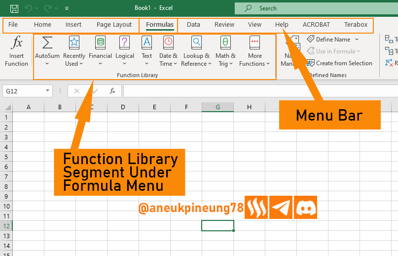
MS Excel has collected advanced formulas into the Formula Library segment of the [Formula] menu. See the following image.

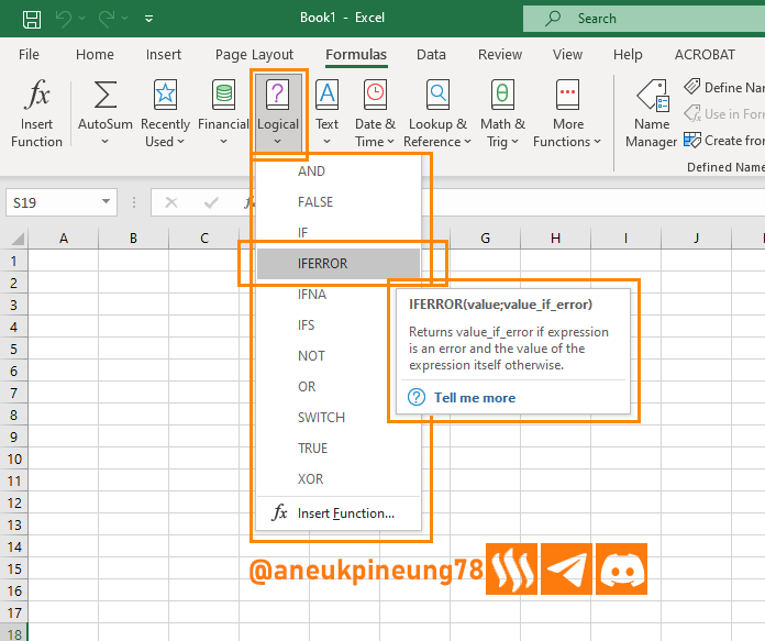
In the Formula Library segment, formulas are grouped into 6 main categories: Financial, Logical, Text, Date & Time, Lookup & Reference, and Math & Trigonometry. There are also Auto Sum and one group that contain miscellaneous functions named More Functions button. The following image shows that when the Logical function button is pressed, a popup containing the logical functions appears, when the user hovers over one of the options, Excel will display a window that provides concise information on that option. This is especially helpful for those who want to learn by themselves.

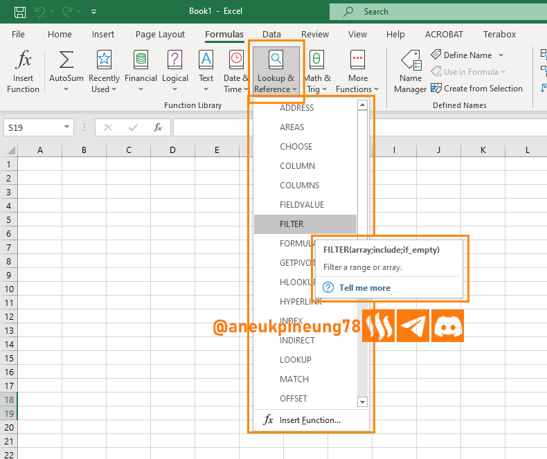
The Lookup & Reference category has more sub menus than the Logical category, the access button is located to the right of the Logical category access button.

Task 2 - Write the IF Function formula to calculate the total, average score, and grade of students given in the table below.

Students	Maths	English	Physics	Chemistry
Simonnwigwe	75	50	84	60
Josepha	76	60	55	90
Kouba01	60	98	85	90
Adeljose	70	60	50	60
Ruthjoe	60	45	80	51
Lhorgic	45	90	70	65
Dove11	70	60	55	75
Ruthjoe	58	70	85	73

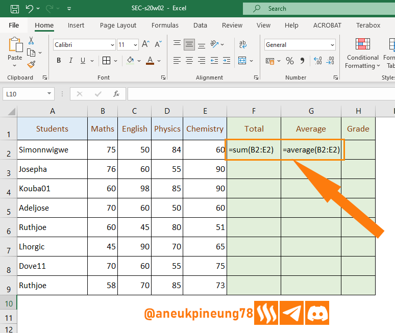
To calculate the total score of each student, I use the SUM function, while for the average, I use the AVERAGE function as shown in the following figure.

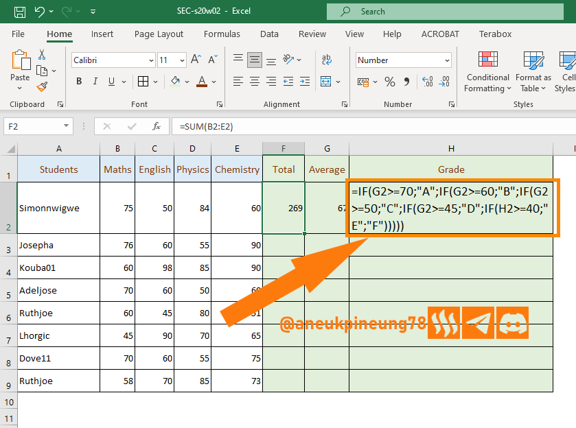
To determine the grade of each student in alphabetical form, I used the grade range as stated in the contest article, which is
70% -100% = A
60% - 69% = B
50% - 59% = C
45% - 49% = D
40% - 44% = E

So the function that I use to calculate Simonnwigwe’s alphabetical grade in cell H2 based on the total score in the cell G2 looks like this:
=IF(G2>=70;"A";IF(G2>=60;"B";IF(G2>=50;"C";IF(G2>=45;"D";IF(H2>=40;"E";"F")))))

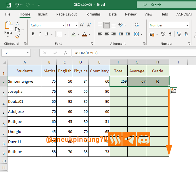
After all the functions worked well on Simonnwigwe's scores, the functions were duplicated for the remaining students.

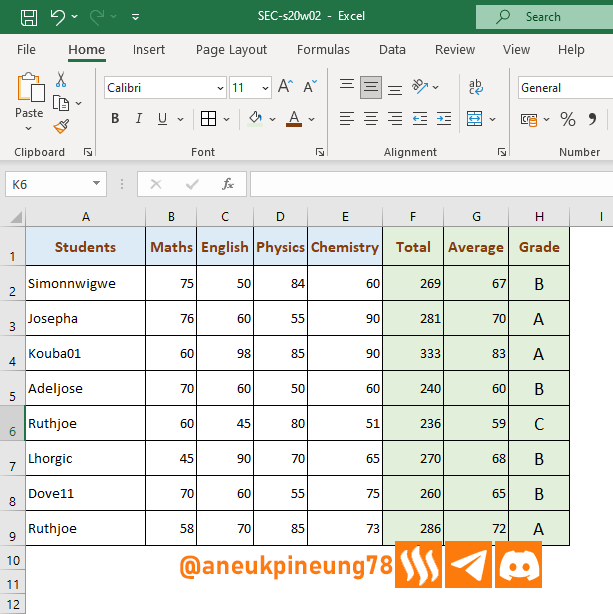
So that the table is obtained as follows.

Task 3 - Briefly discuss four IF function Operators that you have learned and tell us their functions and when we are to use them.

In MS. Excel, the IF operator basically works to find a TRUE or FALSE condition, and then displays a result based on that finding. IF Function Operators can be grouped into four main categories, namely logic operators, comparison operators, mathematical operators, and text operators. Let's discuss them one by one.

Logical Operators, which are operators used to combine multiple conditions into one IF function formula so that MS. Excel will execute complex data based on the logic given.
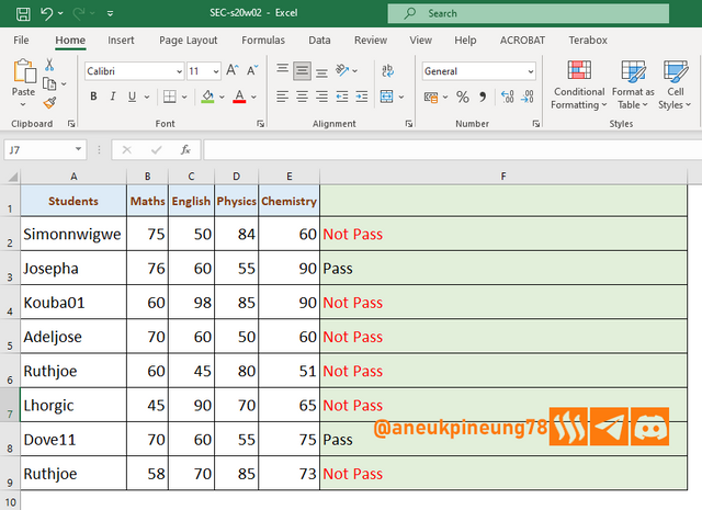
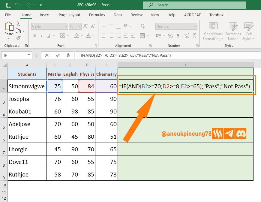
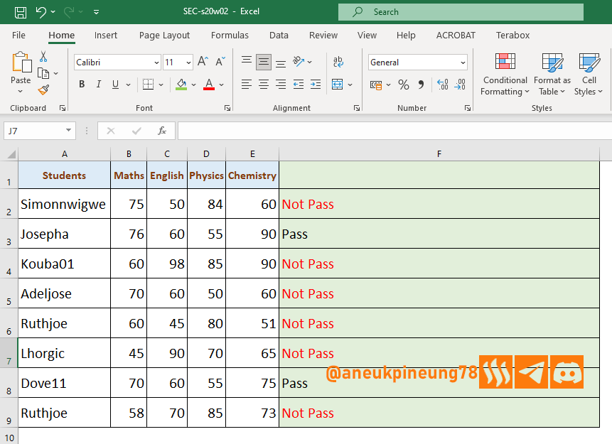
- Examples of this type of operator: OR, NOT, and AND.
- An example of usage in a case based on the data table provided by Professor @josepha, where in the scenario the student must get a minimum score for each subject (Maths: 70, Physics: 80, and Chemistry: 65) in order to PASS. Then the operator used is AND, the formula becomes:
  =IF(AND(B2>=70;D2>=8;E2>=65);“Pass”;“Not Pass”).
  
  Unfortunately, with a fairly high score requirement, only two students PASSED.
Comparison Operator, used to compare two data values. Actually, the example of using this operator is also included in the example above. This operator is simpler than the Logic operator.
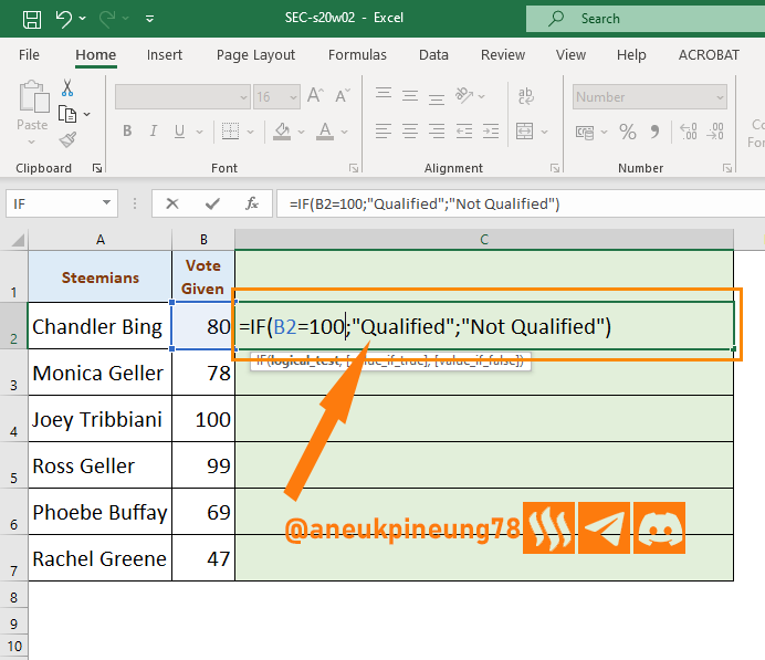
- Included in this category of operators are : =, >, <, >=, <=, <>.
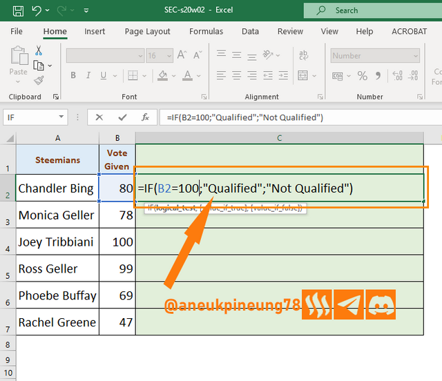
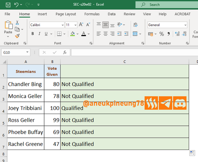
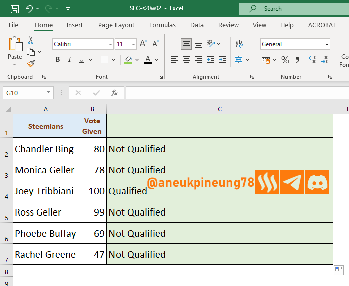
- An example of use case, finding Steemians in a list like the data in the table below who has voted 100 times and marking them as “Qualified”, then the formula becomes:
  =IF(B2=100;“Qualified”;“Not Qualified”)
  
  The result for the operation:
Mathematical Operators, which are operators in the IF function that perform mathematical operations such as addition, subtraction, multiplication, and division.
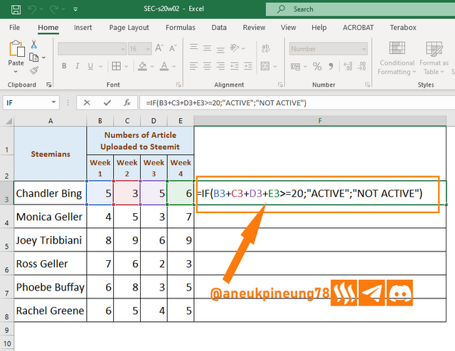
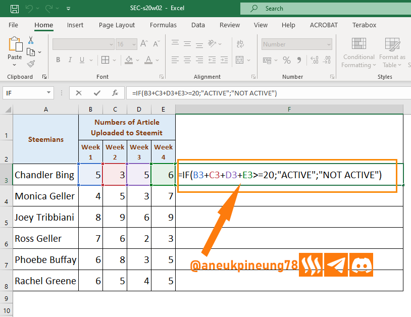
- Included in this category of operators are : + (addition), - (subtraction), * (multiplication), and / (division).
- An example of its use in the scenario of a group of Steemians as in the table below, each of whom is required to write at least 20 articles every four weeks to be labeled ACTIVE. Then the operator used is the addition operator (+) so the formula becomes:
  =IF(B3+C3+D3+E3>=20;“ACTIVE”;“NOT ACTIVE”)
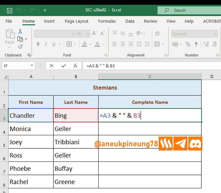
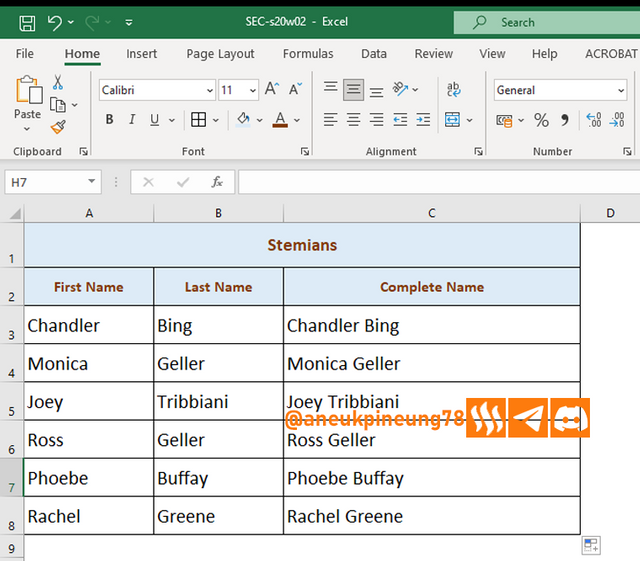
Text Operators, used to manipulate and merge text. There are many text operator, including TEXT, LEFT, RIGHT, and MID. The simplest of this operator cathegory is & which functions to join texts between cells. An example case of using the & operator is seen in the following table which lists the names of six Steemians, the table consists of 3 columns, the first and second columns contain the first and last names, and the user is expected to fill the third column with the full name. Then the formula used is:
=A3 & “ ” & B3

The final result of this operation is as shown in the following image.

Task 4 - Based on the given data below: Create a pivot table that shows (see) total sales by product, by dragging the product to the Rows areas, Region to the Column area, and Sales to the Values area. Please we want to see the steps you take in adding your pivot table.

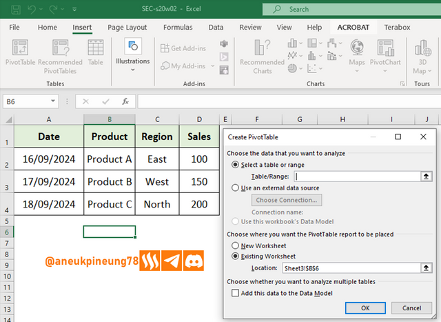
Date	Product	Region	Sales
16/09/2024	Product A	East	100
17/09/2024	Product B	West	150
18/09/2024	Product C	North	200

This is very simple data so it is a very good start if we want to learn Pivot Table in Spreadsheet, especially MS Excel. Here is how I created a Pivot Table from the given data.

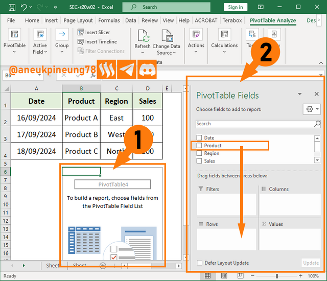
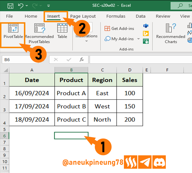
See picture below. After having the data that you want to generate a Pivot Table from, the user must decide where to place the Pivot Table, although actually the Pivot Table that will be generated can also be moved to other areas in the Spreadsheet. In this case, I choose cell B6 (1). Then I select the [Insert] menu on the menu bar (2). Next, in the [Insert] menu, I choose Pivot Table (3).
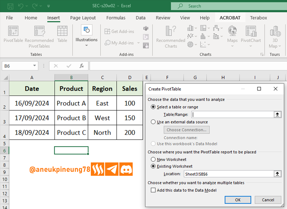
The Create Pivot Table dialog box appears on the right of the screen. The first thing I need to do here is to select the table or cell-range that contains the data I want to create a Pivot Table for.
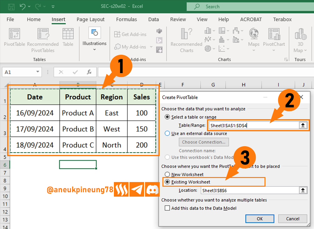
I selected the desired table including the header (1). The table (cell-range) I selected is listed in the Create Pivot Table dialog box (2). In the pointer (3) of the below screenshot, users can specify where the generated Pivot Table will be placed, whether to stay in the selected cell, or want to move to other cells or into a new worksheet. In this case, I do not make any changes about the location of the Pivot Table that I want to generate. I press the [OK] button at the bottom of the dialog box to execute.
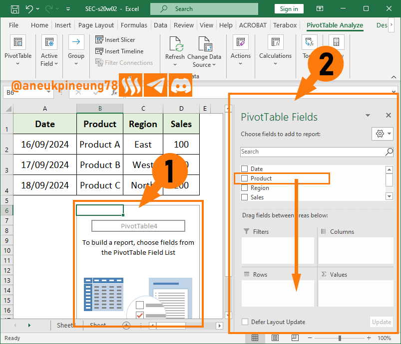
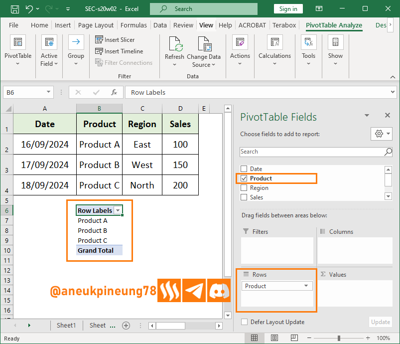
Two dialog boxes appear as shown in the image below. The part that I marked with pointer (1) will show the Pivot Table, but before that, I need to explain first how the characteristics of the Pivot Table that I want, and I have to do it in the second dialog box (2). As directed by Professor @josepha, I drag the Product field to the Rows area.
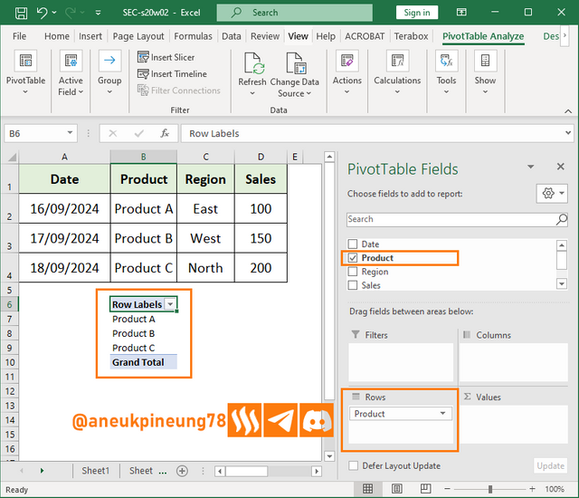
The following image shows the changes in the worksheet after I dragged the Product field to the Rows area.
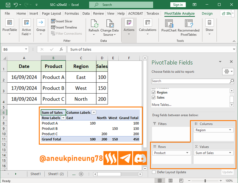
After I dragged the Product field to the Rows area, I continued to carry out the next instruction which was to drag the Region and Sales fields to the Column and Values areas respectively.
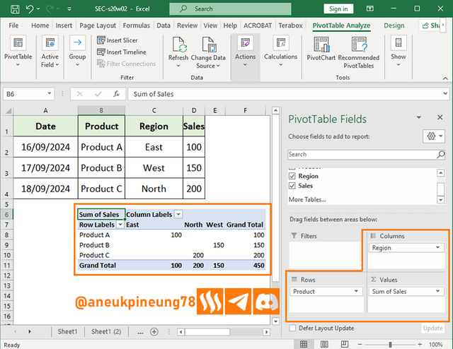
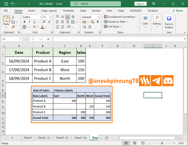
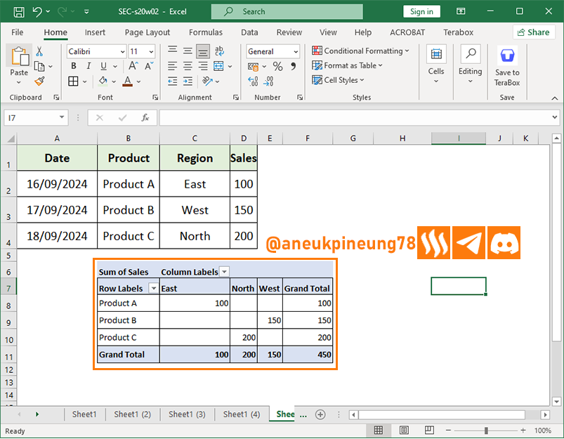
Now I have a simple Pivot Table that I generate from simple data. Pivot Table is just like a normal table, it can be decorated for example by coloring the cells and giving borders. Here is the appearance of the Pivot Table that I created.